The Equations of Ideal Magnetohydrodynamics

Corresponding GitHub Repository

The Theory

The single most ubiquitous set of equations in plasma physics are the ideal magnetohydrodynamics (MHD) equations. These form the foundation of all of plasma physics, including the theory of equilibrium and stability of tokamaks and stellarators, and the proper understanding of everything from space to astrophysical plasmas.

The classical reference for the theory of ideal MHD for fusion application was written by J. P. Freidberg. It contains the derivation of the equations from the more fundamental kinetic equation, the theory of equilibria that underlies many fusion devices, and a theory of general stability. The theory of MHD, both ideal as well as extended (in which non-ideal effects are added), is vast and rich. Much of it was developed in the second half of the last century, and still continues to this day. This theory, and the corresponding numerics, is central to the proper understanding of the bulk motion of plasmas. Recall that plasmas make up greater than 95% of the observable matter in the universe, and hence MHD theory is central to a proper understanding of this universe, in addition to the terrestrial devices we have built in our quest for nuclear fusion.

The key difference between neutral fluids and MHD is that the fluid is electrically conducting, but more importantly, that the magnetic field provides a preferred direction. The structure of the Lorentz force means that the flow of fluid perpendicular to the magnetic field is much more constrained than the flow parallel to it. Further, in the ideal case the magnetic field is frozen into the fluid. That is, as the fluid moves it drags the field with it. Of course, the pressure gradients of the fluid, and field tension, change the flow, leading to a complex interaction between the fluid and the field. The presence of even small non-ideal effects (resistivity and viscosity) can profoundly impact the flows also. In particular, the frozen-in condition is violated, leading to magnetic reconnection and other phenomena that can cause large-scale rearrangement of the the magnetic field. All of this is to say that the structure of the magnetic field is critical to an understanding of plasma physics.

Ideal MHD is a pre-Maxwell theory in the sense that the displacement currents are ignored (hence, no electromagnetic waves) and the plasma is treated as a conducting fluid. The equations consist of the continuity equation

$$ \frac{\partial\rho}{\partial t} + \nabla\cdot(\rho\mathbf{u}) = 0, $$

and the momentum equation

$$ \frac{\partial \mathbf{u}}{\partial t}+\mathbf{u} \cdot \nabla \mathbf{u} +\frac{\nabla p}{\rho} = {\frac{1}{\mu_{0}\rho}(\nabla \times \mathbf{B}) \times \mathbf{B}} $$

where $\mathbf{B}$ is the magnetic field. The right-hand side of this equation is a manifestation of the Lorentz force and how the motion of the plasma is modified due to the magnetic field. The evolution of the magnetic field is determined by the induction equation

$$ \frac{\partial\mathbf{B}}{\partial t} + \nabla\times\mathbf{E} = 0 $$

where $\mathbf{E} = -\mathbf{u}\times\mathbf{B}$ (ideal Ohm’s Law)¹. Finally, for an ideal plasma, the pressure evolves according to

$$ \frac{\partial p}{\partial t} + \mathbf{u}\cdot\nabla p = -\gamma p \nabla\cdot\mathbf{u}. $$

Of course, the magnetic field must be divergence free:

$$ \nabla\cdot\mathbf{B} = 0. $$

This non-conservation form (often also called the gas-dynamic form of the equations) are very useful in analytical work. However, to develop numerical methods we must rewrite them in conservative form. Using some algebraic manipulations we can show that the momentum equation can be written in the conservative form as

$$ \frac{\partial}{\partial t}(\rho\mathbf{u}) + \nabla\cdot \mathbf{T} = 0 $$

where

$$ \mathbf{T} = \rho\mathbf{u}\otimes\mathbf{u} + \left(p + \frac{|\mathbf{B}|^2}{2\mu_0} \right)\mathbf{g} -\frac{1}{\mu_0} \mathbf{B}\otimes\mathbf{B}. $$

is a symmetric second-order tensor describing the momentum flux, and $\mathbf{g}$ is the metric tensor. In index notation we can write this tensor as

$$ T_{ab} = \rho u_a u_b + \left(p + \frac{|\mathbf{B}|^2}{2\mu_0} \right) g_{ab} -\frac{1}{\mu_0} B_a B_b. $$

Some vector-algebra manipulations allow us to derive evolution equations for the kinetic-energy

$$ \frac{\partial}{\partial t} \left( \frac{1}{2}\rho|\mathbf{u}|^2 \right) + \nabla\cdot \left[ \frac{1}{2}\rho|\mathbf{u}|^2\mathbf{u} + \left(p+\frac{|\mathbf{B}|^2}{2\mu_0}\right)\mathbf{u} \right] = \left(p+\frac{|\mathbf{B}|^2}{2\mu_0}\right)\nabla\cdot\mathbf{u} + \frac{1}{\mu_0} \mathbf{u}\cdot \left[ (\mathbf{B}\cdot\nabla)\mathbf{B} \right] $$

the internal energy

$$ \frac{\partial}{\partial t}\left(\frac{p}{\gamma-1}\right) +\nabla\cdot \left(\mathbf{u}\frac{p}{\gamma-1}\right)=-p\nabla\cdot\mathbf{u}, $$

and the magnetic field energy

$$ \frac{\partial}{\partial t}\left(\frac{|\mathbf{B}|^2}{2\mu_0} \right) -\nabla\cdot \left( \frac{1}{\mu_0}(\mathbf{u}\cdot\mathbf{B})\mathbf{B} - \frac{|\mathbf{B}|^2}{2\mu_0}\mathbf{u} \right) = -\frac{|\mathbf{B}|^2}{2\mu_0}\nabla\cdot\mathbf{u} - \frac{1}{\mu_0}\mathbf{u}\cdot[(\mathbf{B}\cdot\nabla)\mathbf{B}]. $$

These evolution equations for the various components of the energy show how energy can be exchanged between various components of the fluid and the field: internal and kinetic energies are exchanged via the fluid compressibility, and kinetic and field energies through a complicated set of terms involving compressibility and currents and the electric field.

If we add the kinetic and internal energy equations together we get an evolution equation for the fluid total energy

$$ \frac{\partial \mathcal{E}_f}{\partial t} + \nabla\cdot \left[ \mathbf{u}(\mathcal{E}_f+p) \right] = \mathbf{E}\cdot\mathbf{J}. $$

where

$$ \mathcal{E}_f = \frac{1}{2} \rho |\mathbf{u}|^2 + \frac{p}{\gamma-1} $$

is the fluid energy. This equation indicates that the fluid exchanges energy with the field via the $\mathbf{E}\cdot\mathbf{J}$ term. This a key feature of a plasma: the field-fluid interaction is always via $\mathbf{E}\cdot\mathbf{J}$ even in more complex plasma models, including the fully kinetic Vlasov-Maxwell model.

Rather neatly, if we add all the components of the energy the right-hand sides all cancel, and we get that the total energy

$$ \mathcal{E} \equiv \mathcal{E}_f + \frac{|\mathbf{B}|^2}{2\mu_0} = \frac{1}{2}\rho|\mathbf{u}|^2 + \frac{p}{\gamma-1} + \frac{|\mathbf{B}|^2}{2\mu_0} $$

evolves as

$$ \frac{\partial \mathcal{E}}{\partial t} + \nabla\cdot \left[ (\mathcal{E}+p^*)\mathbf{u} - \frac{1}{\mu_0}(\mathbf{u}\cdot\mathbf{B})\mathbf{B} \right] = 0 $$

where the total (fluid + magnetic) pressure is defined as

$$ p^* \equiv p + \frac{|\mathbf{B}|^2}{2\mu_0}. $$

Of course, the evolution of the total energy equation is very important. However, one should point out that equally important are the evolution of the components of the energy, as these fundamentally determine energization processes, and also how turbulence manifests in MHD². In fact, it is extremely difficult (perhaps impossible) to develop generic numerical schemes that account for both proper transfer between various components of the energy, and also at the same time account for shocks and other features of compressibility. As nature would have it, these are the cutting-edge regimes of interest for modern, high-energy plasma physics.

As can be imagined, the eigensystem of the ideal MHD equation is not trivial to compute. As in the case of the Euler equations it is best to work with the quasilinear form of the equations. In 1D these become

$$ \frac{\partial}{\partial{t}} \begin{bmatrix} \rho \\ u \\ v \\ w \\ B_x \\ B_y \\ B_z \\ p \end{bmatrix} + \begin{pmatrix}{u} & \rho & 0 & 0 & 0 & 0 & 0 & 0\\ 0 & {u} & 0 & 0 & 0 & -\frac{{B_y}}{{{\mu}_0} \rho} & \frac{{B_z}}{{{\mu}_0} \rho} & \frac{1}{\rho}\\ 0 & 0 & {u} & 0 & 0 & -\frac{{B_x}}{{{\mu}_0} \rho} & 0 & 0\\ 0 & 0 & 0 & {u} & 0 & 0 & -\frac{{B_x}}{{{\mu}_0} \rho} & 0\\ 0 & 0 & 0 & 0 & 0 & 0 & 0 & 0\\ 0 & -{B_y} & -{B_x} & 0 & -{v} & {u} & 0 & 0\\ 0 & {B_z} & 0 & -{B_x} & -{w} & 0 & {u} & 0\\ 0 & p \gamma & 0 & 0 & 0 & 0 & 0 & {u}\end{pmatrix} \frac{\partial}{\partial{x}} \begin{bmatrix} \rho \\ u \\ v \\ w \\ B_x \\ B_y \\ B_z \\ p \end{bmatrix} = 0. $$

Using a computer algebra system we can show that the eigenvalues of the quasilinear matrix are

$$ \begin{align} \lambda^{1,7} &= u \mp c_f \\ \lambda^{2,6} &= u \mp c_a \\ \lambda^{3,5} &= u \mp c_s \\ \lambda^4 &= u \end{align} $$

and $\lambda^8 = 0$. Here, $c_f$ is the fast magnetosonic speed, $c_a$ is the Alfven speed, and $c_s$ is the slow magnetosonic speed respectively. These are defined as

$$ \begin{align} c_a &= \sqrt{\frac{B_x^2}{\mu_0 \rho}} \\ c_f &= \left( \frac{1}{2} \left[ a^2 + \frac{|\mathbf{B}|^2}{\mu_0\rho} + \sqrt{\left(a^2+\frac{|\mathbf{B}|^2}{\mu_0\rho}\right)^2 - 4 a^2 \frac{B_x^2}{\mu_0\rho} } \right] \right)^{1/2} \\ c_s &= \left( \frac{1}{2} \left[ a^2 + \frac{|\mathbf{B}|^2}{\mu_0\rho} - \sqrt{\left(a^2+\frac{|\mathbf{B}|^2}{\mu_0\rho}\right)^2 - 4 a^2 \frac{B_x^2}{\mu_0\rho} } \right] \right)^{1/2} \end{align} $$

where $a = \sqrt{\gamma p/\rho}$ is the sound speed. Unlike the case of the Euler equations the number of modes that can propagated in the ideal MHD system are far more, and more much more complex. Note that when $\mathbf{B} = 0$ the eigenvalues of the ideal MHD equations reduce to that of the Euler equations. The eigenvalues are real as long as $\rho > 0$ and $p > 0$, showing that the ideal MHD equations remain hyperbolic for normal matter.

The expressions for the right- and left-eigenvectors are rather involved. One should consult the paper by Ryu and Jones for the complete list.

The Numerics

The ideal MHD equations, though more complicated, use the same general numerical approach and the Euler equations. Simple Lax fluxes only require an estimate of the fastest eigenvalue (the fast magnetosonic speed), though as with the Euler equations, Lax fluxes can be rather diffusive. And since the eigensystem is more complicated, determining the Roe averages for the ideal MHD is a more involved process. Cargo and Gallice show how one can construct the averaged states to ensure that the flux-jump condition is satisfied³. We should mention that there is a general, alternate approach to constructing fluctuations such that the flux-jump condition is always satisfied: this approach is called the f-wave approach and in one directly splits the jump in flux across an interface rather than the jump in conserved variables. We shall discuss this approach at a later stage.

One major challenge in the ideal MHD equations, analogous the similar problem for Maxwell equations, is numerically preserving the divergence condition, $\nabla \cdot \mathbf{B} = 0$. One manifestation of this issue appears in the eigenvalues: there exists an eigenvalue that has zero speed. There are two ways that divergence condition is preserved: first, using the constrained transport method, and second, by adding a divergence correction as done in the Perfectly Hyperbolic Maxwell equations. At present, Lanyon uses the latter approach but will incorporate both approaches in the future.

In the divergence correction approach we introduce a new scalar field $\psi$ that is used to correct divergence errors. For this we modify the induction equation to add an additional term and introduce a new equation for the evolution of $\psi$:

$$ \begin{align} \frac{\partial\mathbf{B}}{\partial t} + \nabla\times\mathbf{E} + \nabla \psi &= 0 \\ \mathcal{D}(\psi) + \nabla\cdot\mathbf{B} &= 0. \end{align} $$

Here $\mathcal{D}$ is a scalar valued differential operator. There are a number of choices for this operator. See the paper by Dedner et al. The specific choice that Lanyon uses is

$$ \mathcal{D}(\psi) = \frac{1}{c_h^2} \frac{\partial \psi}{\partial t} + \frac{1}{c_p^2} \psi $$

where $c_h$ and $c_p$ are two constants. As one can show, this operator results in a telegraph equation for $\psi$ in which the error propagates through the domain and also damps. Often one sets $c_p = \infty$ and uses open boundary conditions for $\psi$ (independent of the boundary conditions for the other variables) so the errors leave the domain in a finite time.

We finally mention that for many production problems one needs to use constrained transport as well as apply divergence cleaning. Lanyon will eventually construct such schemes to ensure divergence errors are truly minimized.

The Proofs

Like the Euler equations, the ideal MHD equations are nonlinear. However, unlike Euler equations they also contain additional physics, in particular the interaction with a magnetic field. Lanyon can generate the specifications, the proofs and the C kernels in just under 8 minutes, including for 1D, 2D and 3D ideal MHD equations, including for divergence correction terms.

In all, Lanyon generates almost 50,000 lines of Lean code and more than 30,000 line of formally verified C kernels. One reason for the large number of lines is the complexity of the eigensystem listed above. For example, one can see the complexity of the generated code from the $x$-direction eigenvalue definitions. These complex definition are then used in theorems, for example, to prove the hyperbolicity of the $y$-direction fluxes. Other theorems need equally complex definitions and tactics, taking just under four minutes to typecheck the Lean code.

The Results

We look at two problems that typify the type of solutions one obtains with the ideal MHD equations. For a full description of the steps needed to run Lanyon see the Research Note on Advection-Diffusion Equation where we describe the Lanyon commands and the sequence in which they must be run.

The first simulation is a classical 1D shock problem, the Brio-Wu problem. Plots from the exact solution are given in the Formulary. We first create a solver using the deepthought command:

/deepthought Create a solver for the 1D ideal MHD equations

We use the deepthought rather than the specify command as the ideal MHD equation is sufficiently complicated that it requires a more complex reasoning model to generate the DSL specification for the solver. Once the solver is generated, verified and compiled, then we can run the simulation:

/simulate Simulate a 1D Brio-Wu shock problem for ideal MHD on 1024 grid.

This command will create the simulation driver for the Brio-Wu problem and run the simulation, creating a set of plots. An example of the generated plot is shown below.

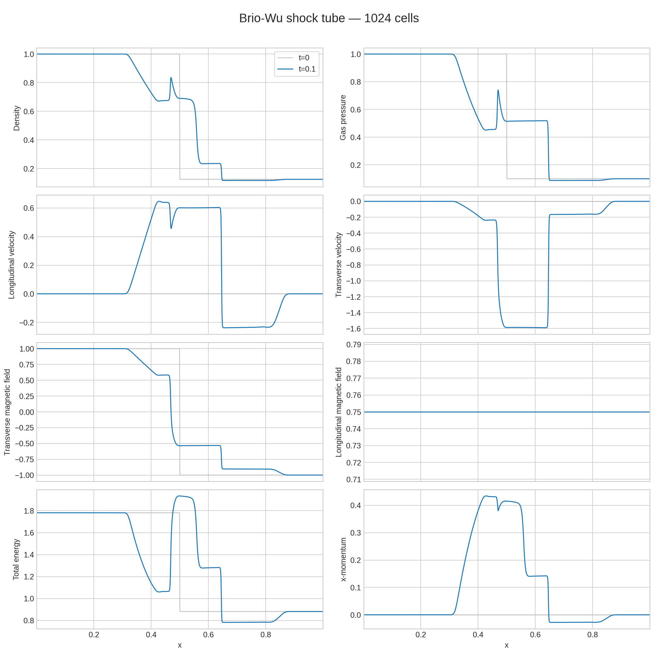
The solution shows a rarefaction wave, contact discontinuity as well as a shock. Across the contact the pressure remains continuous while the density shows a jump. Note the spike-like feature: this is the compound wave, which does not appear in the Euler shock solutions and is unique to ideal MHD. The other notable feature is the shock in the magnetic field. This occurs as the field is frozen into the fluid, and hence when the fluid shocks so does the field.

Next, we generate a 2D solver. To get numerically stable solutions we need to include divergence corrections as described above.

/deepthought Create a solver for the 2D ideal MHD equations. Use a divergence preserving scheme

This will create a solver using the Dedner method described above, allowing the divergence errors to be propagated out of the domain at a finite speed bounded by the fastest eigenvalue.

A classic 2D problem is the Orsag-Tang problem: in this problem an initial set of smooth fluid and field configuration is perturbed. The prompt to run the simulation is:

/simulate Simulate a 2D Orsag-Tang vortex problem on a 1024 x 1024 grid on a 1 x 1 domain. Keep density and pressure plots and movies as GIFs. Run to t=0.5

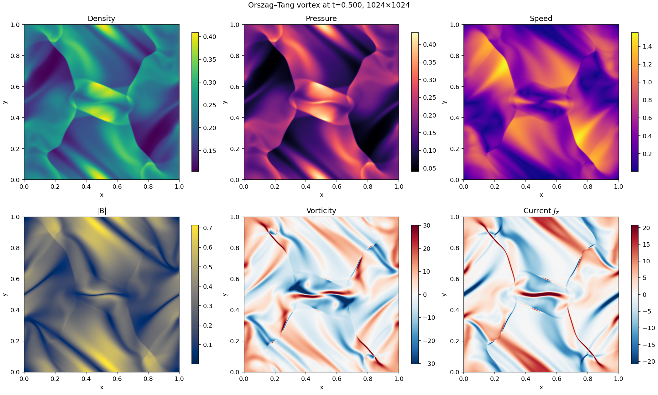
The initial condition is unstable and the perturbation drives the simulation nonlinear. Complex shocks propagate, and current sheets (internal boundary-layers in the current) form. When small non-ideal effects are added the thinning current-sheets are accompanied by magnetic reconnection, in which the magnetic field changes topology. Note that the ideal MHD model does not allow the field topology to change, and hence to properly understand magnetic reconnection one needs to add non-ideal effects or use more complex models, for example, the multifluid, multi-moment models. Lanyon supports such extended plasma models, eventually including the full Vlasov-Maxwell system, and we will present reconnection results later.

The next simulation shows Lanyon’s ability to do MHD flows over general geometries. For this we use the same 2D ideal MHD solver created above and then simulate supersonic flow over a conducting cylinder. We add an initial uniform out-of-plane magnetic field. The full prompt to the simulate command is:

/simulate Simulate the Mach 2 flow over a conducting cylinder. Add an initial out-of-plane magnetic field

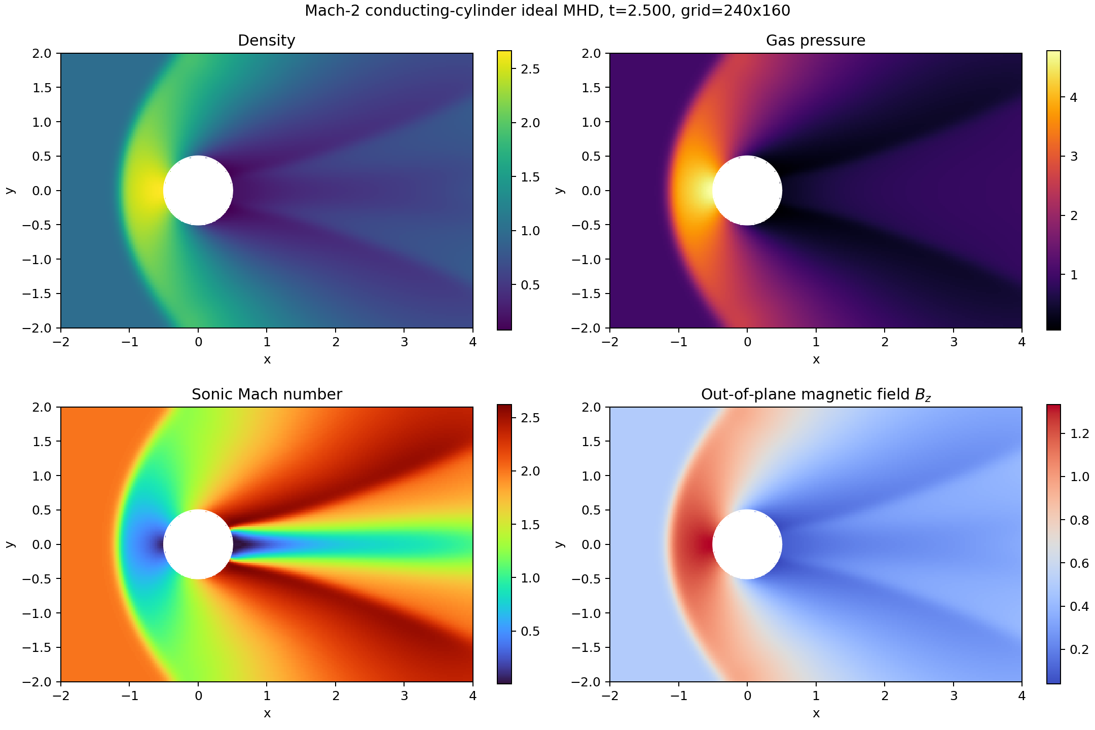
As the flow impinges on the cylinder it will drag the field with it as seen in the bottom right panel of the above figure. The gradient of the magnetic field pressure ($\mathbf{B}^2/2\mu_0$) exerts an additional force on the incoming flow. This results in a larger shock stand-off-distance than in a neutral flow problem.

References and Footnotes